Curves: natural spline vs PCHIP, overshoot, luma and LUT baking

A curve editor looks like a drawing tool, but underneath it is one decision with visible consequences: how to draw a smooth line through the points you placed. My colour engine offers three answers and uses two of them in different places. This part covers why, what overshoot does to an image, how a master RGB curve differs from a luma curve (with measurements from the engine), and what happens to a curve when it is baked into a LUT.

What a curve is in this engine

A curve has 2 to 16 points, both axes 0…1, with x strictly increasing. The ends are kept; clicking adds a point, arrows move the selected one by 1/255 (10/255 with Shift), Delete removes an interior point. In the pipeline from part 1, the master curve is applied to each encoded RGB channel first, then the R, G and B curves, and the luma curve later, in the photo stage. There are three interpolation modes: linear, smooth (PCHIP) and spline (natural cubic). One mode serves master, R, G and B together; the luma curve is always PCHIP. A project saved before the mode field existed keeps linear, because that is what it was made with.

The coefficients are compiled once per grade. In the pixel loop there is a segment search over at most 15 intervals and a Horner evaluation, with no allocation and no validation:

// native/src/color.cpp
double sample(double input) const {
  if (input <= x.front()) return y.front();
  if (input >= x.back()) return y.back();
  std::size_t index = 0;
  while (input > x[index + 1]) ++index;
  if (input == x[index + 1]) return y[index + 1];
  const double t = (input - x[index]) / (x[index + 1] - x[index]);
  if (mode == CurveMode::linear) return y[index] + (y[index + 1] - y[index]) * t;
  const double value = ((d[index] * t + c[index]) * t + b[index]) * t + y[index];
  return mode == CurveMode::spline ? clamp(value) : value;
}

The last line is the whole story of this article in one expression: only the spline needs a clamp.

The natural cubic spline, and its price

The spline mode solves for second derivatives M_i at the points. With h_i = x_(i+1) − x_i and secant slopes d_i, the system is tridiagonal:

h_(i−1)·M_(i−1) + 2(h_(i−1) + h_i)·M_i + h_i·M_(i+1) = 6(d_i − d_(i−1)),   M_0 = M_(n−1) = 0

The engine solves it with the Thomas algorithm when the points change, then stores per-segment cubic coefficients in local t. Value, first derivative and second derivative are continuous at every point, which makes it the softest shape you can put through a set of points. New RGB curves use it by default. I checked it against SciPy's natural CubicSpline as an external oracle: the JavaScript copy agrees to 6.7e-16, and the C++ engine agrees with the JavaScript copy to 3e-13, including a curve strong enough to clip.

The price is overshoot. A natural spline does not know that the output must stay within 0…1, or that a curve through rising points should keep rising.

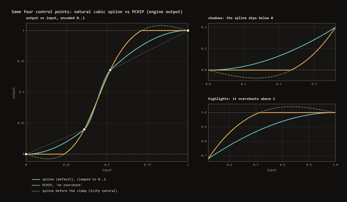
These are the four points I used for the browser check of the spline mode: (0, 0), (0.36, 0.2), (0.52, 0.68), (1, 1). Before the clamp the spline reaches −0.037 and 1.041. On a dense ramp of 10,001 inputs it is below 0 for inputs up to 0.235 and above 1 from 0.714. After the SDR clamp that becomes a flat black over roughly the first 60 input codes and a flat white over the top 73. Inside those flat areas the curve is no longer C², and it is no longer strictly increasing either: shadow detail below code 60 becomes one value. On this curve the spline and PCHIP differ by up to 31 output codes, at input 0.70. That is not a styling difference in how the line looks; it is a different photograph.

PCHIP: no new extremes, one derivative fewer

The smooth mode is PCHIP, the piecewise cubic Hermite interpolant with Fritsch–Butland tangents (Fritsch and Butland, 1984), which satisfy the monotonicity conditions of Fritsch and Carlson, 1980. Each interior tangent is a weighted harmonic mean of the two neighbouring secants, and it is set to zero when the secants have different signs or one of them is zero:

m_k = (w1 + w2) / (w1/d_(k−1) + w2/d_k),   w1 = 2h_k + h_(k−1),   w2 = h_k + 2h_(k−1)
m_k = 0  if d_(k−1)·d_k <= 0

The end tangents use a one-sided three-point estimate with limits on sign and size, the same rule SciPy's PchipInterpolator uses. The result passes through every point, has a continuous first derivative, and never creates a new extreme between neighbouring points. If the points rise, the curve rises. The second derivative can jump at a point, which is the one derivative fewer in the heading; in practice it shows as a slightly less rounded bend.

The maths suite samples a monotone PCHIP curve at 1,025 inputs and checks that no step goes down; the smallest step it measured is 2.2e-6. On the curve in the figure, PCHIP's smallest step is 1.5e-6, while the clamped spline has steps of exactly zero. In the editor the PCHIP mode is labelled "no overshoot".

So why keep both? Because they answer different requests. For a gentle bend through points well inside the range, the spline gives the softer shape and the difference is small. For a strong S-curve close to black and white, PCHIP keeps shadow and highlight gradation that the spline throws away. The mode is one switch, and it stays saved with the project.

Master RGB curve versus luma curve

A master RGB curve applies the same function to encoded R, G and B. A grey stays grey. A colour does not keep its channel ratios, so a contrast curve also raises saturation and turns hue a little. The luma curve is the answer to "change the tone and leave the colour alone". It works on linear luminance with BT.709 weights, Y = 0.2126R + 0.7152G + 0.0722B, and rebuilds RGB so that the new luminance is exactly f(Y):

// native/src/photo_color.cpp
std::array<double, 3> linear{srgbToLinear(levelled[0]), srgbToLinear(levelled[1]), srgbToLinear(levelled[2])};
// Luma curve: RGB' = RGB * (f(Y) - f(0)) / Y + f(0), so Y' = f(Y) exactly (see photo-color.mjs).
const double y = lumaOf(linear);
const double mappedY = luma.sample(y);
if (y > kLumaFloor) {
  for (double& channel : linear) channel = channel * (mappedY - lumaBlack) / y + lumaBlack;
  linear = clipToLuminance(linear, mappedY);
} else {
  linear = {mappedY, mappedY, mappedY};
}

Both lines around the gain are fixes. The first version scaled RGB by f(Y)/Y. With a lifted black, f(0) > 0, that gain explodes near black: a blue one code above zero became 255. Treating the lift as a neutral offset, f(0) added to all three channels, keeps it a lift. The second fix is for channels that land outside 0…1. Clipping them one by one missed the target luminance by up to 0.137 and turned hue by up to 13.6°. The engine now uses the ClipColor construction from ISO 32000-1 §11.3.5.3, part of the PDF specification's non-separable blend modes: out-of-range channels are pulled towards the grey of the same luminance, so Y' = f(Y) holds even where a channel would clip. The maths suite measures the luminance error of the luma curve below 1e-15.

To see what this buys, I ran one S-curve both ways through the engine. The master curve was a PCHIP S-curve on encoded values; the luma curve was built so that greys come out the same, within 0.25 of a code.

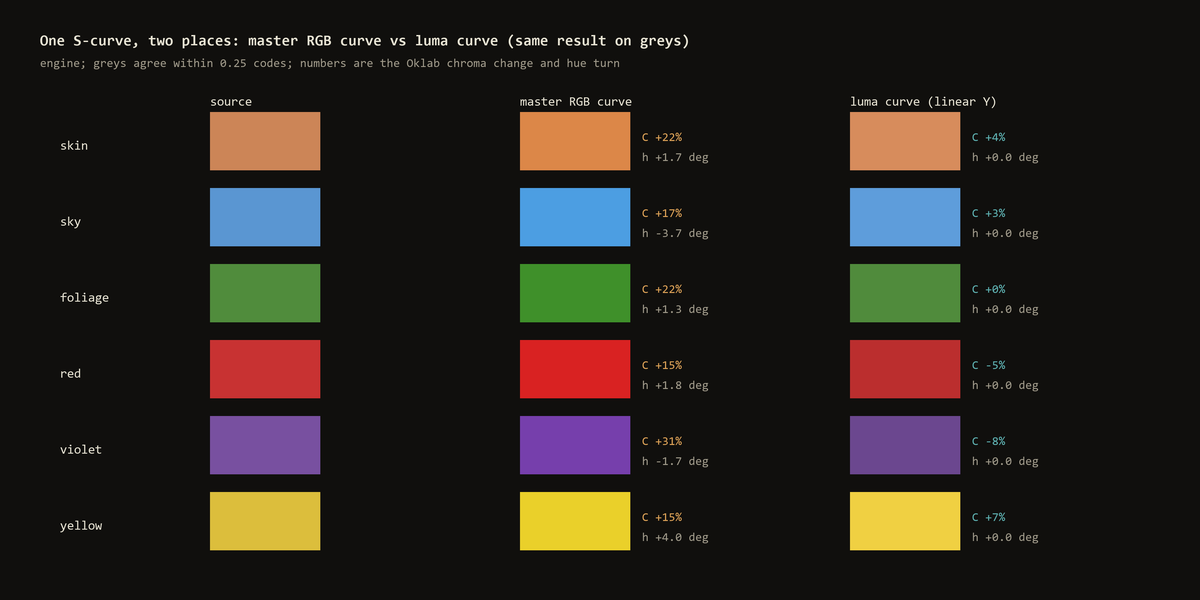
On six test colours the master RGB curve raised Oklab chroma by 15 to 31% and turned hue by up to 4.0°. The luma curve changed chroma by −8% to +7% and turned hue by 0.0°. Chroma still moves a little because Oklab chroma follows lightness even at constant chromaticity. Capture One documents the same intent for its Luma curve, contrast without a saturation increase; Adobe's Camera Raw point curve offers composite and per-channel curves. Neither publishes a formula, and mine is my own.

One consequence for the interface: the luma curve lives on a linear luminance scale, so the same point coordinates mean different tones than on the master curve. The editor shows it on its own scale and draws no channel overlays for it.

Perceptual-axis curves: designed, not built

A candidate curve tool is written down but not in the panel or the engine. It puts three curves on Oklab axes, L2 = fL(L), a2 = fa(a), b2 = fb(b), with the centres locked, fa(0) = 0 and fb(0) = 0, so any neutral stays neutral; the lock can be released only by an explicit action with a warning that neutrals will shift. The result mixes in through a mask weight m and strength s, out = (1 − s·m)·source + s·m·OklabToRgb(L2, a2, b2), and two checks are shown before it applies: a broken neutral lock and colours that leave the gamut. Gamut compression there must be an explicit mode, never a silent clamp.

Baking curves into a LUT

Everything global in a grade (tone, colour, curves, the input LUT, colour protection) depends only on the input RGB, so it can be exported as a 3D CUBE or a Hald image. Spatial edits such as clarity or dehaze depend on neighbours and position, and the engine refuses to put them into a LUT; the editor exports the colour-only part of such a grade only after you explicitly confirm that the spatial edits will be left out. Baking samples the full transform at N³ lattice points, N from 2 to 65, red fastest.

At the lattice points the CUBE matches the engine: 3e-8 for a spline-only grade at 33³, which is float precision, and 1.7e-6 for a grade using every global control, inside the review's 2e-6 threshold. Between the points it is interpolation, and it is honest to say how much. On that full grade, 4,096 off-lattice samples gave an RMS error of 0.010 (about 2.6 codes) at 33³ and 0.0054 at 65³. The worst single sample was far worse: at 33³ a near-yellow input came out with its blue channel 0.53 too high, and at 65³ the worst sample was still 0.27 off. The review marked export as HOLD, meaning the CUBE is an approximation of this grade, not a copy, and the native image or the project is the faithful output. The engine has a verify call that returns exactly these two numbers, maximum and RMS over 4,096 samples, for whatever grade is being exported. Part 2 shows the same effect on a single Levels set, where a 65³ lattice missed by about 23 codes next to black.

Precision

The colour transform runs in double and rounds once, when it writes 8-bit or 16-bit output. Curves are evaluated analytically per pixel, not through an internal 1D table. The main window works on the browser's 8-bit sRGB canvas, and a steep curve on an 8-bit source spreads 256 input levels over a wider range, which is where banding comes from. The lab window reads 16-bit PNG without passing it through the canvas, exports 16-bit PNG, and can apply an ordered 8×8 dither when it has to reduce to 8 bits. The dither depends on pixel position, so it is never part of a LUT. None of this restores gradation that a JPEG never had; it only stops the edit from destroying more.

The curve drag had a problem of its own, measured in time rather than codes. In the first version, a 61-event drag drew the curve once, 3.56 s after the first move. Now the graph redraws on every animation frame independently of processing, the editor sends one preview at a time to the C++ engine and keeps only the latest parameters waiting, and the curve histogram is cached per source image. The same drag draws 61 curve frames, the first after 33.9 ms, and the first processed image after 267 ms. One Undo still reverts the whole drag.

Limits

• The natural spline is the default for RGB curves and it can clip at the ends; PCHIP is the mode for strong curves near black and white.
• Luma is always PCHIP, on linear luminance, and does not claim parity with Capture One or Adobe.
• Perceptual-axis curves are a design, not a feature.
• A baked CUBE of a complex grade is an approximation; check its maximum and RMS error before sending it anywhere.

Next part: hue, saturation and lightness by colour. If the native side interests you more than colour, the on-device C++ retouching plugin is on happyin.ai.